• Linear Regression with one variable
  • Notion
  • Hypothesis
  • Cost function
  • Gredient descent
• Linear Regression with multiple variables
  • Notion
  • Hypothesis derivation
  • Hypothesis
  • Cost function
  • Gradient descent
  • Feature Scaling
  • Mean normalization
  • Learning rate
    • “Debugging”: How to make sure gradient descent is working correctly.
    • How to choose learning rate
  • Normal Equation
• Linear Algebra:
  • Matrices and vectors
  • Addition and scalar multiplication
    • Matrix Addition
    • Scalar Multiplication
  • Matrix-vector multiplication
  • Matrix-matrix multiplication
  • Matrix multiplication properties
  • Inverse and transpose
• Octave Tutorial
  • Basic operations
  • Moving data around
  • Computing on data
  • Plotting data
  • Control statements: for, while, if statements
  • Vectorial implementation

Linear Regression with one variable

Notion

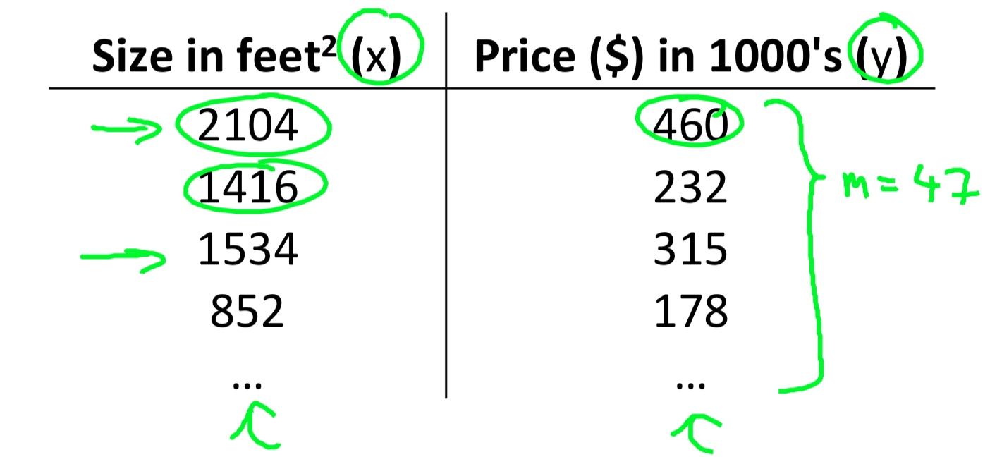
• m = Number of training examples
• x’s = “input” variable / features
• y’s = “output” variable / “target” variable

Hypothesis

\[ h_{\theta}(x) = \theta_0 + \theta_1x \]

Cost function

\[
J(\theta)
= \frac{1}{2m} \sum_{i=1}^m (h_\theta(x^{(i)}) - y^{(i)})^2
= \frac{1}{2m} \sum_{i=1}^m (\theta_0+\theta_1x^{(i)} - y^{(i)})^2
\]

Gredient descent

\[
\theta_j = \theta_j - \alpha \frac{\partial}{\partial\theta_j} J(\Theta) \\
= \theta_j - \alpha \frac{\partial}{\partial\theta_j} (\frac{1}{2m} \sum_{i=1}^m (h_\theta(x^{(i)}) - y^{(i)})^2) \\
= \theta_j - \alpha \frac{1}{m} \sum_{i=1}^m (h_\theta(x^{(i)}) - y^{(i)})(x^{(i)}_j)
\]

• j = 0

\[
\theta_0 = \theta_0 - \alpha \frac{1}{m} \sum_{i=1}^m(\theta_0+\theta_1x^{(i)}-y^{(i)})
\]

• j = 1

\[
\theta_1 = \theta_1 - \alpha \frac{1}{m} \sum_{i=1}^m(\theta_0+\theta_1x^{(i)}-y^{(i)})x^{(i)}
\]

(simultaneously update \(\theta_j\) for all j)

Linear Regression with multiple variables

Notion

• \(n\) = number of features
• \(x^{(i)}\) = input of \(i^{th}\) training example
• \(x^{(i)}_j\) = input of \(i^{th}\) training example 's \(j^{th}\) feature.
• \(x^{(2)}_3\) = 2

Hypothesis derivation

• Previousely: \( h_{\theta}(x) = \theta_0 + \theta_1x \)
• New algorithm: \( h_{\theta}(x) = \theta_0 + \theta_1x_1 + \theta_2x_2 + \theta_3x_3 \)

\(
X =
\begin{bmatrix} x_0\\x_1\\x_2\\\vdots\\x_n \end{bmatrix}
\in R^{n+1}
\)

\(
\Theta =
\begin{bmatrix} \theta_0\\\theta_1\\\theta_2\\\vdots\\\theta_n \end{bmatrix}
\in R^{n+1}
\)

• For convenience of notation, define \(x_0=1\)

\(
h_{\theta}(x)
= \theta_0x_0 + \theta_1x_1 + \theta_2x_2 + \theta_3x_3
= \Theta^TX
\)

Hypothesis

\[
\begin{align}
h_{\theta}(x)
&= \Theta^TX \\
&= \theta_0x_0 + \theta_1x_1 + \theta_2x_2+ \cdots + \theta_nx_n
\end{align}
\]

Cost function

\[
\begin{align}
J(\theta)
&= J(\theta_0, \theta_1, \cdots, \theta_n) \\
&= \frac{1}{2m} \sum_{i=1}^{m}(h_\theta(x^{(i)})-y^{(i)})^2
\end{align}
\]

Gradient descent

\[
\begin{align}
\theta_j &= \theta_j - \alpha \frac{\partial}{\partial\theta_j} J(\Theta) \\
&= \theta_j - \alpha \frac{\partial}{\partial\theta_j} (\frac{1}{2m} \sum_{i=1}^m (h_\theta(x^{(i)}) - y^{(i)})^2) \\
&= \theta_j - \alpha \frac{1}{m} \sum_{i=1}^m (h_\theta(x^{(i)}) - y^{(i)})(x^{(i)}_j)
\end{align}
\]

• j = 0

\[
\theta_0 = \theta_0 - \alpha \frac{1}{m} \sum_{i=1}^m(\theta_0+\theta_1x^{(i)}-y^{(i)})(x^{(i)}_0)
\]

• j = 1

\[
\theta_1 = \theta_1 - \alpha \frac{1}{m} \sum_{i=1}^m(\theta_0+\theta_1x^{(i)}-y^{(i)})x^{(i)}(x^{(i)}_1)
\]

……

Feature Scaling

• Make sure features are on a similar scale.
• Get every feature into approximately a \(-1 \leq x_i \leq 1\) range.

Mean normalization

Replace \(x_i\) with \(x_i-\mu_i\) to make features have approximately zero mean
(Do not apply to ).

E.g.
\[ x_1 = \frac{size-1000}{2000} \]
\[ x_2 = \frac{bedrooms-2}{5} \]

\[x_1 = \frac{x_1-\mu_1}{\sigma_1}\]
\[x_2 = \frac{x_2-\mu_2}{\sigma_2}\]

Learning rate

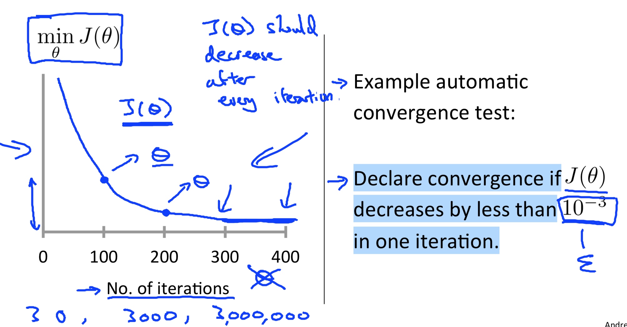
While doing gradient decent

\[
\theta_j = \theta_j - \alpha \frac{\partial}{\partial\theta_j} J(\Theta)
\]

“Debugging”: How to make sure gradient descent is working correctly.

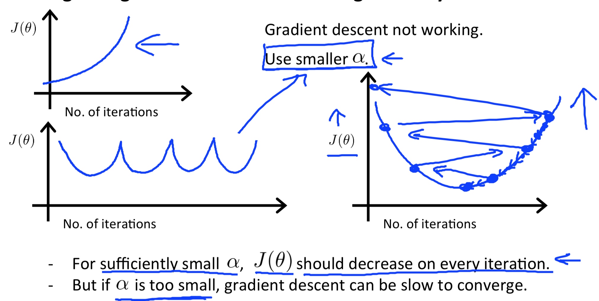
How to choose learning rate

Summary:

• If \(\alpha\) too small: slow convergence
• If \(\alpha\) too large: \(J(\theta)\) may not decrease on every iteration; may not converge.

To choose \(\alpha\), try

\(\cdots, 0.001, 0.003, 0.01, 0.03, 0.1, 0.3, 1, \cdots\)

Normal Equation

Normal equation: Method to solve for analy2cally.

\[ \theta = (X^TX)^{-1}X^Ty \]

	Gradient Descent	Normal Equation
1	Need choose \(\alpha\)	No need to choose \(\alpha\)
2	Need many iterations	Do not need to iterate
3	Works well even n is large	Need to compute \((X^TX)^{-1}\), time complexity O(n3)
4		Slow if n is very large

Linear Algebra:

Matrices and vectors

• Matrix:
• Dimension of matrix:
• Matrix Elements
• Vector

Addition and scalar multiplication

Matrix Addition

Scalar Multiplication

Matrix-vector multiplication

Matrix-matrix multiplication

Matrix multiplication properties

Inverse and transpose

• Inverse
• Transponse

Octave Tutorial

Basic operations

Moving data around

Computing on data

Plotting data

Control statements: for, while, if statements

Vectorial implementation

\[
\begin{split}
&\theta_j = \theta_j - \alpha \frac{\partial}{\partial\theta_j} J(\Theta) \\
&= \theta_j - \alpha \frac{\partial}{\partial\theta_j} (\frac{1}{2m} \sum_{i=1}^m (h_\theta(x^{(i)} - y^{(i)}))^2) \\
&= \theta_j - \alpha \frac{\partial}{\partial\theta_j} (\frac{1}{2m} \sum_{i=1}^m (\theta_0+\theta_1x^{(i)} - y^{(i)})^2) \\
&= \theta_j - \alpha (\frac{1}{m} \sum_{i=1}^m (1+x^{(i)}))
\end{split}
\]